Introduction to Concentration Inequalities: From Markov to McDiarmid

0. Introduction

In probability and statistics, we often care less about the value of a random quantity itself than about how far it can deviate from its typical value.

As an example, consider the sample mean

of independent and identically distributed (i.i.d.) random variables $X_1, \dots, X_n$. If $\mathbb{E}[|X_1|] < \infty$, the law of large numbers states that $\bar{X}_n$ converges to the expectation $\mu := \mathbb{E}[X_1]$ with probability $1$ as $n \to \infty$. In real data analysis, however, $n$ is finite. What we want to know is how small the following probability is for a given $n$ and $\varepsilon > 0$:

Inequalities that bound this probability from above in terms of $n$, $\varepsilon$, and properties of the distribution (such as its range or variance) are called concentration inequalities.

The central limit theorem also describes the fluctuations of $\bar{X}_n$, but it states the shape of the distribution in the limit $n \to \infty$ and says nothing about the size of the error at a finite $n$. Concentration inequalities give bounds that hold as they are at a finite $n$.

Running example: estimating a success probability

Throughout this article, we compare the inequalities on the following problem.

We use the following two settings, each with $\delta = 0.05$ and $\delta = 10^{-6}$:

• (A) $p = 0.5$, $\varepsilon = 0.05$: the variance of one trial, $p(1-p)$, takes its maximum value $1/4$.
• (B) $p = 0.01$, $\varepsilon = 0.005$: successes are rare, and the variance $p(1-p) \approx 0.0099$ is small.

First, we examine the distribution of $\hat{p}$ in setting (A) with Python. The following code generates $\hat{p}$ $10^5$ times for each of $n = 10, 100, 1000$ and plots histograms.

import numpy as np
import matplotlib.pyplot as plt

rng = np.random.default_rng(0)
p, eps, trials = 0.5, 0.05, 100_000

for n in [10, 100, 1000]:
    # Success rates of n trials with success probability p, repeated trials times
    p_hat = rng.binomial(n, p, size=trials) / n
    # Fraction with an error of eps or more (1e-12 guards against rounding errors)
    miss = np.mean(np.abs(p_hat - p) >= eps - 1e-12)
    bins = (np.arange(n + 2) - 0.5) / n  # bins of width 1/n centered at k/n
    plt.hist(p_hat, bins=bins, density=True, histtype="step", lw=2,
             label=f"$n = {n}$ ({miss:.3f})")

plt.axvspan(p - eps, p + eps, color="gray", alpha=0.2)
plt.xlim(0.2, 0.8)
plt.xlabel(r"$\hat p$")
plt.ylabel("Density")
plt.legend(loc="upper left")
plt.show()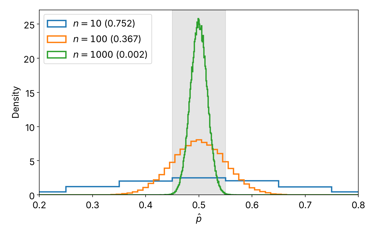

As Figure 1 shows, the distribution of $\hat{p}$ concentrates around $p = 0.5$ as $n$ grows, and the fraction of runs with an error of $0.05$ or more drops from $0.752$ at $n = 10$ to $0.367$ at $n = 100$ and $0.002$ at $n = 1000$. Concentration inequalities give upper bounds on this fraction without computing the distribution in detail.

All figures in this article, including Figures 2 and 5 whose code is not shown here, can be regenerated with code/concentration/make_figures.py.

Roadmap

The inequalities covered in each section and the information each one uses are as follows:

1. Markov's inequality (Section 2): nonnegativity and the expectation
2. Chebyshev's inequality (Section 3): the variance
3. The Chernoff method (Section 4): the moment generating function
4. Hoeffding's inequality (Section 5): independence and the range
5. Bernstein's inequality (Section 6): independence, the range, and the variance
6. McDiarmid's inequality (Section 7): independence and a bound on how much the output changes when one input changes

Section 8 compares the results for the running example, and Section 9 introduces tools for cases where the assumptions fail. An inequality in a later section is not always stronger than one in an earlier section. Which inequality gives the smallest bound depends on the available assumptions and the conditions of the problem.

1. Notation and basics

Tail probabilities and the union bound

The probability that a random variable $X$ deviates from its expectation by $t > 0$ or more is called a tail probability. Depending on the direction of the deviation, there are three kinds:

• Upper tail probability: $\Pr(X - \mathbb{E}[X] \geq t)$
• Lower tail probability: $\Pr(X - \mathbb{E}[X] \leq -t)$
• Two-sided tail probability: $\Pr(|X - \mathbb{E}[X]| \geq t)$

Concentration inequalities give upper bounds on these tail probabilities (tail bounds). Because $\Pr(A \cup B) \leq \Pr(A) + \Pr(B)$ holds for any events $A$ and $B$ (the union bound), the two-sided tail probability is at most the sum of the upper and lower tail bounds. Therefore, when the same bound holds for both the upper and the lower tail, the two-sided bound has a factor of $2$.

2. Markov's inequality

Markov's inequality bounds a tail probability using only nonnegativity and the expectation. Every other inequality in this article uses it somewhere in its proof.

Proof.　Because $X \geq 0$ a.s., the inequality $X \geq t \mathbf{1}_{\{X \geq t\}}$ holds with probability $1$ (the right-hand side is $t$ when $X \geq t$ and $0$ otherwise). Taking expectations of both sides gives $\mathbb{E}[X] \geq t \Pr(X \geq t)$, and dividing by $t$ gives Theorem 1. $\square$

Setting $t = c\, \mathbb{E}[X]$ with $c > 0$ gives $\Pr(X \geq c\, \mathbb{E}[X]) \leq 1/c$. For example, the probability that a nonnegative random variable is at least $10$ times its expectation is at most $1/10$. In exchange for the weak assumptions, the bound decreases only as $1/t$.

Bounding the indicator function with nonnegative functions

The proof bounds the indicator function $\mathbf{1}_{\{X \geq t\}}$ from above by a nonnegative function and takes the expectation. In general, if a random variable $Y$ and a nonnegative function $\varphi$ satisfy $\varphi(y) \geq \mathbf{1}_{\{y \geq t\}}$ for every value $y$ that $Y$ can take, then

Different choices of $\varphi$ give different inequalities (Figure 2).

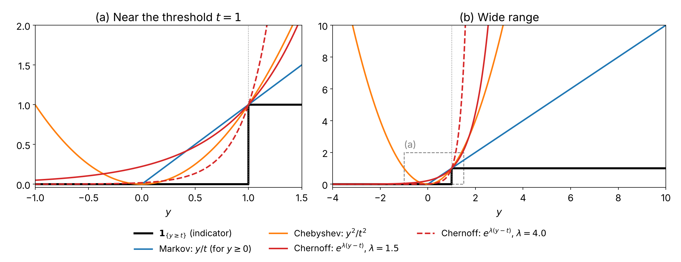
• Markov's inequality (Section 2) uses $\varphi(y) = y/t$ with a nonnegative $Y = X$.
• Chebyshev's inequality (Section 3) uses $\varphi(y) = y^2/t^2$ with $Y = X - \mathbb{E}[X]$. This $\varphi$ is also at least $1$ for $y \leq -t$, so it bounds the two-sided tail probability at once.
• The Chernoff method (Section 4) uses $\varphi(y) = e^{\lambda(y - t)}$ with $\lambda > 0$ and $Y = X - \mathbb{E}[X]$.

The closer $\varphi$ is to the indicator function where $Y$ is likely to take values, the smaller the bound. In the Chernoff method, $\lambda$ controls the shape of $\varphi$. Near $t$ in Figure 2(a), the curve for $\lambda = 4$ is closer to the indicator function for $y < t$ than the curve for $\lambda = 1.5$, but it grows faster for $y > t$. Section 4 optimizes this $\lambda$.

The wide range in Figure 2(b) shows how differently the functions grow far from $t$. Markov's $y/t$ is linear in $y$, and Chebyshev's $y^2/t^2$ grows in both directions away from $0$. The Chernoff function $e^{\lambda(y - t)}$ approaches $0$ as $y$ decreases but grows exponentially for $y > t$. Therefore, for $\mathbb{E}[\varphi(Y)]$ to be finite in the Chernoff method, the moment generating function of $Y$ (Section 4) must be finite; that is, the upper tail of $Y$ must decay at least exponentially fast.

3. Chebyshev's inequality

Chebyshev's inequality uses the variance to bound how far a random variable deviates from its expectation.

Proof.　Applying Markov's inequality to the nonnegative random variable $(X - \mathbb{E}[X])^2$ gives

Application to the sample mean

Suppose that $X_1, \dots, X_n$ are pairwise uncorrelated with a common expectation $\mu$ and a common variance $\sigma^2$. Then $\operatorname{Var}(\bar{X}_n) = \sigma^2/n$, and Theorem 2 gives

The calculation of $\operatorname{Var}(\bar{X}_n)$ uses only the additivity of variance, so uncorrelatedness, which is weaker than independence, is enough.

Running example.　The variance of one trial is $\sigma^2 = p(1-p)$, so the right-hand side is at most $\delta$ if

In setting (A) with $\delta = 0.05$, this gives $n \geq 2{,}000$. Because the required $n$ is proportional to $1/\delta$, it becomes $n \geq 10^8$ for $\delta = 10^{-6}$.

4. The Chernoff method

The bound from Chebyshev's inequality decreases only polynomially in $t$. Using an exponential function gives bounds that decrease exponentially in $t$. This technique is called the Chernoff method or the Cramér–Chernoff method (Chernoff, 1952; Boucheron et al., 2013, §2.2).

General form

The function $\lambda \mapsto \mathbb{E}[e^{\lambda X}]$ of $\lambda \in \mathbb{R}$ is called the moment generating function (MGF) of $X$. In this article, we use the logarithm of the MGF of the centered random variable:

If $\psi_X(\lambda)$ is finite for $\lambda > 0$, then, because $x \mapsto e^{\lambda x}$ is increasing, Markov's inequality gives

Because this holds for every $\lambda > 0$ with $\psi_X(\lambda) < \infty$, minimizing the right-hand side over $\lambda$ gives

This bound is called the Chernoff bound. Any upper bound on $\psi_X$ turns it into a concrete bound. The lower tail probability is bounded by applying the same argument to $-X$.

Sums of independent random variables

With the exponential function, the MGF of a sum of independent random variables factors into the product of their MGFs. If $X_1, \dots, X_n$ are independent, then

and taking logarithms gives $\psi_{S_n}(\lambda) = \sum_{i=1}^n \psi_{X_i}(\lambda)$. Therefore, bounds on each $\psi_{X_i}$ give a bound on the tail probability of the sum $S_n$. Hoeffding's inequality in Section 5 and Bernstein's inequality in Section 6 are derived in this way.

Sub-Gaussian random variables

For a normal random variable with variance $\nu$, $\psi_X(\lambda) = \nu\lambda^2/2$ holds with equality. In other words, a sub-Gaussian random variable is one whose centered MGF is at most that of a normal distribution. For a sub-Gaussian $X$, the function $\lambda t - \nu\lambda^2/2$ attains its maximum $t^2/(2\nu)$ at $\lambda = t/\nu$, so the Chernoff method gives

Because the definition also covers $\lambda < 0$, the same bound holds for the lower tail, and the two-sided bound has a factor of $2$ (Boucheron et al., 2013, §2.3).

In addition, if independent $X_i$ are sub-Gaussian with variance parameters $\nu_i$, then $\psi_{S_n} = \sum_i \psi_{X_i}$ implies that $S_n$ is sub-Gaussian with variance parameter $\sum_{i=1}^n \nu_i$. Section 5 uses this property to derive Hoeffding's inequality.

A relative-error bound for sums of Bernoulli random variables

Applying the Chernoff method to sums of Bernoulli random variables gives a bound on the error relative to the expectation (Mitzenmacher & Upfal, 2017, Chapter 4).

The second inequality in the first display follows from $\log(1 + \eta) \geq 2\eta/(2 + \eta)$, which holds for $\eta \geq 0$. This theorem measures the error by its ratio $\eta$ to the expectation $m$. When $m$ is small compared with $n$, it can give a smaller bound than Hoeffding's inequality in Section 5 (see Section 8).

Running example.　If $p_i = p$, then $m = np$. The event $|\hat{p} - p| \geq \varepsilon$ is the event that a relative error of $\eta := \varepsilon/p$ occurs upward or downward. When $\eta < 1$, the lower-tail exponent $\eta^2 m/2$ is at least the upper-tail exponent $\eta^2 m/(2 + \eta)$, so combining both tails gives

The right-hand side is at most $\delta$ if $n \geq (2 + \eta)\log(2/\delta) / (\eta^2 p)$; in setting (B) ($\eta = 0.5$) with $\delta = 0.05$, this gives $n \geq 3{,}689$.

5. Hoeffding's inequality

When independent random variables take values in known bounded intervals, the Chernoff method yields Hoeffding's inequality (Hoeffding, 1963). The key is the following lemma, which shows that bounded random variables are sub-Gaussian.

For a proof, see Chapter 2 of Boucheron et al. (2013).

Proof.　By Hoeffding's lemma, each $X_i$ is sub-Gaussian with variance parameter $(b_i - a_i)^2/4$. As shown in Section 4, the independent sum $S_n$ is sub-Gaussian with variance parameter $\nu := \sum_{i=1}^n (b_i - a_i)^2/4$, so

Sample mean and required sample size

If each $X_i \in [a, b]$ a.s. with a common expectation $\mu$, setting $t = n\varepsilon$ in Theorem 4 gives

For fixed $\varepsilon$, this bound decreases exponentially in $n$. Chebyshev's bound $\sigma^2/(n\varepsilon^2)$ in Section 3 decreases only as $1/n$.

Setting the right-hand side to $\delta$ and solving gives two equivalent forms:

• If $n \geq \dfrac{(b - a)^2}{2\varepsilon^2} \log\dfrac{2}{\delta}$, then $\Pr(|\bar{X}_n - \mu| \geq \varepsilon) \leq \delta$.
• For any $n$, with probability at least $1 - \delta$, $|\bar{X}_n - \mu| < (b - a)\sqrt{\dfrac{\log(2/\delta)}{2n}}$.

Running example.　Because $X_i \in [0, 1]$, the condition is $n \geq \log(2/\delta)/(2\varepsilon^2)$. In setting (A), this gives $n \geq 738$ for $\delta = 0.05$ and only $n \geq 2{,}902$ for $\delta = 10^{-6}$. The required $n$ grows in proportion to $\log(1/\delta)$, so the gap from Chebyshev's inequality, whose $n$ grows in proportion to $1/\delta$, widens as $\delta$ decreases. In setting (B), however, even $\delta = 0.05$ requires $n \geq 73{,}778$. Because Hoeffding's inequality uses only the range $[0, 1]$, it cannot reflect that the variance in (B), $p(1-p) \approx 0.0099$, is about $1/25$ of $1/4$, the maximum variance of a random variable on $[0, 1]$. Bernstein's inequality in Section 6 addresses this limitation.

6. Bernstein's inequality

Hoeffding's inequality uses only the range. For random variables whose values mostly lie near the expectation despite a wide range, Bernstein's inequality, which also uses the variance, gives a smaller bound (Boucheron et al., 2013, §2.8).

Two rates of decay

How fast the bound decays depends on which of the two terms in the denominator $V + Mt/3$ is larger. Because $V + Mt/3 \leq 2\max\{V, Mt/3\}$,

• For $t \leq 3V/M$, the exponent is at least $t^2/(4V)$. Like the tail of a normal distribution with variance $V$, the bound decays with an exponent proportional to $t^2$.
• For $t > 3V/M$, the exponent is at least $3t/(4M)$. Like the tail of an exponential distribution, the bound decays with an exponent proportional to $t$.

Sample mean and comparison with Hoeffding's inequality

Suppose that $X_1, \dots, X_n$ are i.i.d. with $\mathbb{E}[X_i] = \mu$, $\operatorname{Var}(X_i) = \sigma^2$, and $|X_i - \mu| \leq M$ a.s. Substituting $V = n\sigma^2$ and $t = n\varepsilon$ into Theorem 5 gives

When $X_i \in [a, b]$, the variance is at most $(b - a)^2/4$. Replacing $\sigma^2$ with this maximum and ignoring $M\varepsilon/3$ gives the exponent $2n\varepsilon^2/(b - a)^2$, which equals the exponent of Hoeffding's bound in Section 5. In this sense, Hoeffding's inequality is a bound that assumes the largest possible variance. Comparing the two exponents shows that Bernstein's bound is smaller when $\sigma^2 + M\varepsilon/3 < (b - a)^2/4$.

Running example.　With $\sigma^2 = p(1-p)$ and $M = \max\{p, 1 - p\}$, the condition is

In setting (B) with $\delta = 0.05$, this gives $n \geq 3{,}409$, about $1/22$ of Hoeffding's $73{,}778$. In setting (A), $\sigma^2 = 1/4$ is already the maximum, so $n \geq 763$, slightly more than Hoeffding's $738$.

7. McDiarmid's inequality

Sections 5 and 6 dealt with sums of random variables. McDiarmid's inequality, also called the bounded differences inequality, deals with general functions $f(X_1, \dots, X_n)$ of independent random variables, not only sums (McDiarmid, 1989; Boucheron et al., 2013, §6.1).

The bounded differences condition expresses stability: changing only the $i$-th input changes the output by at most $c_i$.

Relation to Hoeffding's inequality

Consider the sum $f(x_1, \dots, x_n) = \sum_{i=1}^n x_i$ with $x_i \in [a_i, b_i]$. Changing the $i$-th input changes the sum by at most $b_i - a_i$, so substituting $c_i = b_i - a_i$ into Theorem 6 gives the same formula as Theorem 4 (Hoeffding's inequality). McDiarmid's inequality extends the assumption of Hoeffding's inequality from "a sum of independent bounded random variables" to "a function that is stable under changes of each input."

Example: uniform deviation of the empirical distribution function

As an example of a function that is not a sum, let $X_1, \dots, X_n$ be i.i.d. with cumulative distribution function $F$, and consider the largest difference between $F$ and the empirical distribution function $F_n(x) := \frac{1}{n} \sum_{i=1}^n \mathbf{1}_{\{X_i \leq x\}}$:

$Z$ is called the Kolmogorov–Smirnov statistic and is used to test whether a sample follows the distribution $F$. Changing one $X_i$ changes $F_n(x)$ by at most $1/n$ at every $x$, so it also changes the supremum $Z$ by at most $1/n$. With $c_i = 1/n$, we have $\sum_{i=1}^n c_i^2 = 1/n$, and Theorem 6 gives

The exact distribution of $Z$ at a finite $n$ is not easy to compute, but this bound holds for every $F$.

We check this bound with Python. The following code draws $n = 100$ and $n = 1000$ samples from the uniform distribution $\mathrm{Uniform}(0, 1)$ (so $F(x) = x$) $10^4$ times, computes $Z$, and estimates $\Pr(Z - \mathbb{E}[Z] \geq t)$. It uses the mean over the $10^4$ runs as $\mathbb{E}[Z]$.

import numpy as np
import matplotlib.pyplot as plt

rng = np.random.default_rng(0)
reps = 10_000
s = np.linspace(0, 1.5, 151)  # the horizontal axis is sqrt(n) * t

for n in [100, 1000]:
    # Draw reps samples of size n from Uniform(0, 1) and sort each sample
    u = np.sort(rng.random((reps, n)), axis=1)
    i = np.arange(1, n + 1)
    # Z = sup_x |F_n(x) - x| (largest gap between the empirical CDF and F(x) = x)
    z = np.maximum(i / n - u, u - (i - 1) / n).max(axis=1)
    tail = [np.mean(z - z.mean() >= x / np.sqrt(n)) for x in s]
    plt.semilogy(s, tail, lw=2, label=f"Simulation ($n = {n}$)")

plt.semilogy(s, np.exp(-2 * s**2), "k--", lw=2,
             label=r"McDiarmid bound $e^{-2nt^2}$")
plt.ylim(1e-4, 1.5)
plt.xlabel(r"$\sqrt{n}\,t$")
plt.ylabel(r"$\Pr(Z - \mathbb{E}[Z] \geq t)$")
plt.legend()
plt.show()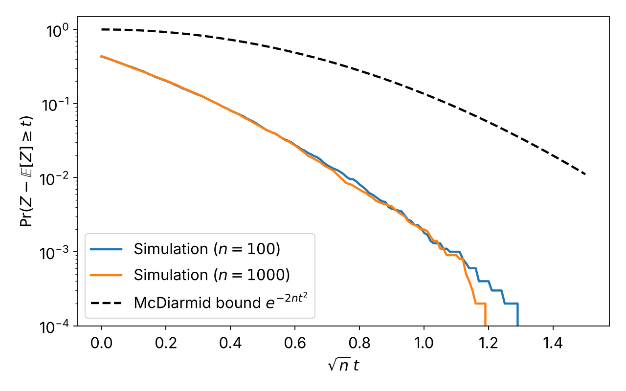

With $\sqrt{n}\, t$ on the horizontal axis, the bound $e^{-2nt^2} = e^{-2(\sqrt{n}\, t)^2}$ becomes a single curve that does not depend on $n$. In Figure 3, the simulation results for $n = 100$ and $n = 1000$ almost coincide, and both lie below the bound. In other words, the fluctuations of $Z - \mathbb{E}[Z]$ are of order $1/\sqrt{n}$, and McDiarmid's inequality captures this order correctly.

The same structure appears in machine learning. Let $\mathcal{G}$ be a set of loss functions with values in $[0, 1]$, and consider $\sup_{g \in \mathcal{G}} \left|\frac{1}{n} \sum_{i=1}^n g(X_i) - \mathbb{E}[g(X_1)]\right|$; the same argument shows the bounded differences condition with $c_i = 1/n$. This quantity is the largest gap between the average loss on the training data and the expected loss, and it is used to bound the generalization error. In generalization bounds based on Rademacher complexity, McDiarmid's inequality keeps this quantity close to its expectation, and the expectation is then bounded by the Rademacher complexity (Bartlett & Mendelson, 2002).

8. Comparison and choosing an inequality

Results for the running example

Table 1 summarizes the sample sizes derived in Sections 3 to 6 that guarantee $\Pr(|\hat{p} - p| \geq \varepsilon) \leq \delta$. For comparison, it also shows the sample sizes actually required, computed numerically from the binomial distribution. Chebyshev's and Bernstein's inequalities use the true variance $p(1-p)$. In practice, $p$ is unknown, so an upper bound on the variance is used instead (for example, $0.0099$ if $p \leq 0.01$ is known).

Table 1: Lower bounds on the sample size $n$ that guarantee $\Pr(|\hat{p} - p| \geq \varepsilon) \leq \delta$

The last row gives the smallest $n$ such that $\Pr(|\hat{p} - p| \geq \varepsilon) \leq \delta$ holds for every sample size at or above it. For $n$ such that $n(p \pm \varepsilon)$ is an integer, the event includes the boundary value with $|\hat{p} - p| = \varepsilon$, so the exact probability does not decrease monotonically in $n$. For this reason, the row shows approximate values.

The following code plots the exact $\Pr(|\hat{p} - p| \geq \varepsilon)$ from the binomial distribution and the bound from each inequality as functions of $n$.

import numpy as np
import matplotlib.pyplot as plt
from scipy.stats import binom

def exact_tail(n, p, eps):
    """Pr(|S/n - p| >= eps) for S ~ Bin(n, p)"""
    # 1e-9 guards against floating-point rounding errors
    upper = np.ceil(n * (p + eps) - 1e-9)
    lower = np.floor(n * (p - eps) + 1e-9)
    return binom.sf(upper - 1, n, p) + binom.cdf(lower, n, p)

def bounds(n, p, eps):
    """Upper bounds on Pr(|p_hat - p| >= eps) from each inequality"""
    var, M, eta = p * (1 - p), max(p, 1 - p), eps / p
    return {
        "Chebyshev": var / (n * eps**2),
        "Chernoff (relative)": 2 * np.exp(-eta**2 * n * p / (2 + eta)),
        "Hoeffding": 2 * np.exp(-2 * n * eps**2),
        "Bernstein": 2 * np.exp(-n * eps**2 / (2 * (var + M * eps / 3))),
    }

settings = [("A", 0.5, 0.05, 4000), ("B", 0.01, 0.005, 20000)]
fig, axes = plt.subplots(1, 2, figsize=(14, 5.6), sharey=True)
for ax, (label, p, eps, n_max) in zip(axes, settings):
    n = np.arange(10, n_max + 1, 10)
    ax.semilogy(n, exact_tail(n, p, eps), "k", lw=1.2, label="Exact (binomial)")
    for name, value in bounds(n, p, eps).items():
        ax.semilogy(n, np.minimum(value, 1), lw=2.2, label=name)
    ax.axhline(0.05, color="gray", ls="--")
    ax.set(title=rf"({label}) $p = {p}$, $\varepsilon = {eps}$",
           xlabel="$n$", xlim=(0, n_max), ylim=(1e-10, 2))
axes[0].set_ylabel(r"$\Pr(|\hat p - p| \geq \varepsilon)$")
axes[1].legend(loc="lower left")
plt.show()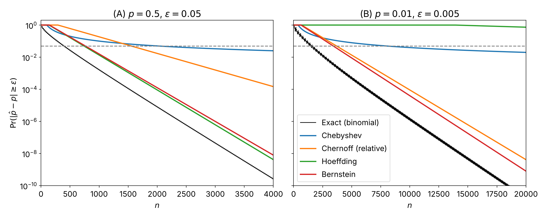

Table 1 and Figure 4 show three points:

1. Growth as $\delta$ decreases: Reducing $\delta$ from $0.05$ to $10^{-6}$ multiplies the $n$ from Chebyshev's inequality by $5 \times 10^4$, because it is proportional to $1/\delta$. The $n$ from the exponential bounds (Chernoff, Hoeffding, and Bernstein) is proportional to $\log(2/\delta)$ and grows only by a factor of about $3.9$. In Figure 4, this difference appears as straight lines (exponential decay) versus a flattening curve ($1/n$ decay).
2. Small variance: In setting (B), Bernstein's inequality, which uses the variance, and the Chernoff bound, which uses the error relative to the expectation, give an $n$ about $20$ times smaller than Hoeffding's inequality, which uses only the range. For $\delta = 0.05$, even Chebyshev's inequality gives a smaller $n$ than Hoeffding's inequality.
3. Conservativeness: Every bound requires more samples than actually needed; even the smallest bound is about $1.2$–$1.8$ times the exact value in setting (A) and about $1.3$–$2.1$ times in setting (B). Concentration inequalities do not use the detailed shape of the distribution, and they are conservative to that extent.

Choosing an inequality

Table 2 summarizes the assumptions and bounds of each inequality.

Table 2: Assumptions and bounds of each inequality

The following list gives rough guidelines for choosing an inequality:

• Only nonnegativity and the expectation are known → Markov's inequality
• The variance is known, but independence cannot be assumed → Chebyshev's inequality (it also applies to sample means of uncorrelated variables)
• The MGF can be computed → the Chernoff method directly
• A sum of independent Bernoulli random variables, with the error measured relative to the expectation → the relative-error Chernoff bound
• A sum of independent bounded random variables, with no information on the variance → Hoeffding's inequality
• A sum of independent bounded random variables whose variance is small compared with the range → Bernstein's inequality
• A function that is not a sum, but on which each input has a small effect → McDiarmid's inequality

9. When the assumptions fail

Dependent random variables

Markov's and Chebyshev's inequalities do not require independence. In contrast, Hoeffding's, Bernstein's, and McDiarmid's inequalities in the forms shown in this article assume independence and do not apply as they are to dependent random variables. There are exceptions: Hoeffding (1963) showed that the same bounds as for sampling with replacement also hold for sampling without replacement from a finite population, where the samples are not independent. In addition, the Azuma–Hoeffding inequality applies to martingales with bounded increments (Azuma, 1967). The proof in the column of Section 7 is based on the same martingale argument as this inequality.

Unbounded random variables

Unbounded random variables can also concentrate. For example, a normal distribution is unbounded but, as shown in Section 4, sub-Gaussian. Sub-exponential random variables form a class that contains the sub-Gaussian ones and also allows heavier tails, and Bernstein-type bounds hold for them (Vershynin, 2018, Chapter 2). Even for distributions without a finite MGF, finite higher moments give bounds that decrease polynomially in $t$, by the method of Section 2.

10. Conclusion

As Figure 5 shows, the inequalities in this article follow from Markov's inequality along two paths.

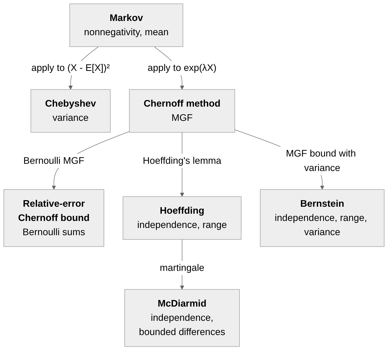
• Markov → Chebyshev: Applying Markov's inequality to the squared deviation bounds tail probabilities by the variance.
• Markov → Chernoff method → Hoeffding, Bernstein, McDiarmid: Applying Markov's inequality to an exponential function and bounding the MGF gives bounds that decrease exponentially. McDiarmid's inequality uses a martingale decomposition to extend these bounds to functions other than sums.

Every one of these inequalities answers the same question: how far can a quantity computed from finitely many samples deviate from its expectation? As the running example in Section 8 shows, which inequality gives the smallest bound depends on the available assumptions (variance, range, independence, and stability of the function) and on the conditions of the problem.

References

• Azuma, K. (1967). Weighted sums of certain dependent random variables. Tohoku Mathematical Journal, 19(3), 357–367.
• Bartlett, P. L., & Mendelson, S. (2002). Rademacher and Gaussian complexities: Risk bounds and structural results. Journal of Machine Learning Research, 3, 463–482.
• Boucheron, S., Lugosi, G., & Massart, P. (2013). Concentration Inequalities: A Nonasymptotic Theory of Independence. Oxford University Press.
• Chernoff, H. (1952). A measure of asymptotic efficiency for tests of a hypothesis based on the sum of observations. The Annals of Mathematical Statistics, 23(4), 493–507.
• Hoeffding, W. (1963). Probability inequalities for sums of bounded random variables. Journal of the American Statistical Association, 58(301), 13–30.
• McDiarmid, C. (1989). On the method of bounded differences. In Surveys in Combinatorics, 1989 (London Mathematical Society Lecture Note Series 141), 148–188. Cambridge University Press.
• Mitzenmacher, M., & Upfal, E. (2017). Probability and Computing: Randomization and Probabilistic Techniques in Algorithms and Data Analysis (2nd ed.). Cambridge University Press.
• Vershynin, R. (2018). High-Dimensional Probability: An Introduction with Applications in Data Science. Cambridge University Press.