0. Introduction

Recently, machine learning models, including deep learning, have undergone dramatic evolution. However, behind this progress lay "mysteries" that could not be fully explained by classical statistics.

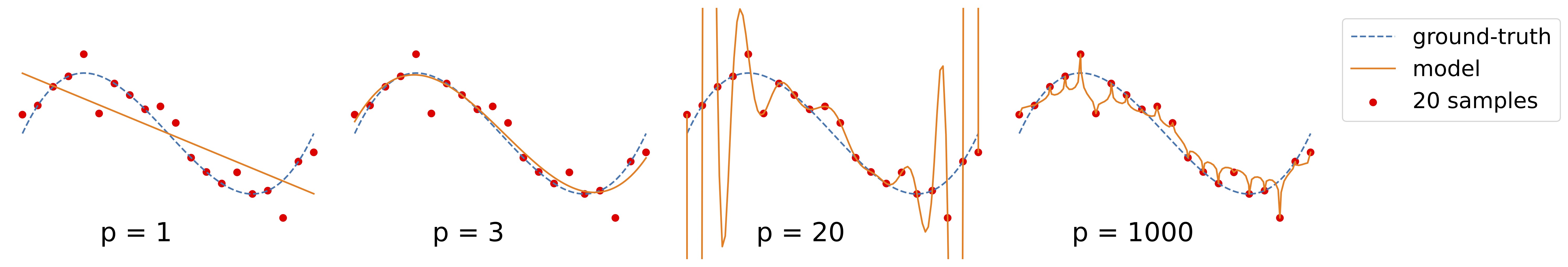
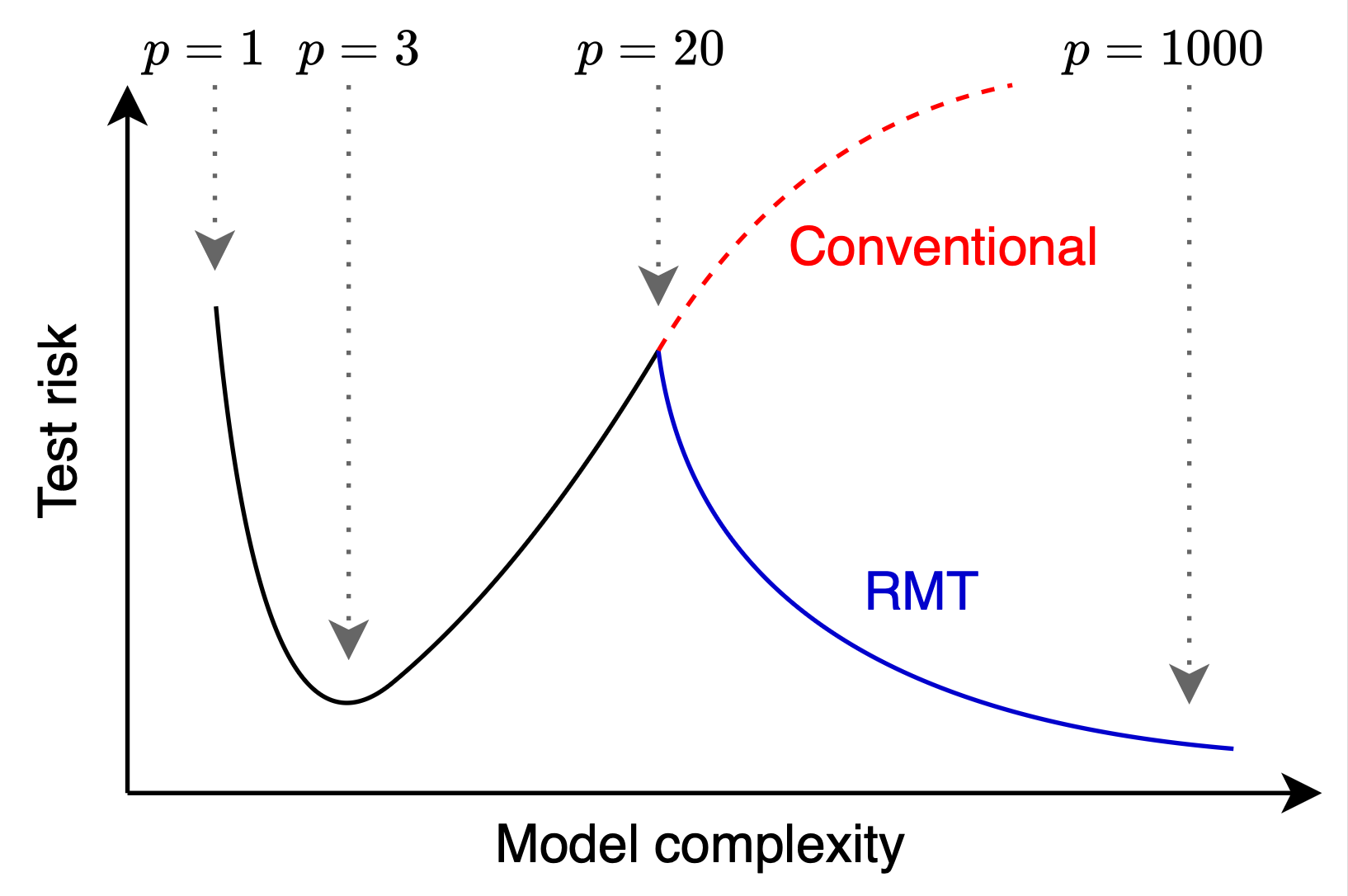
According to the common sense of the bias-variance tradeoff based on conventional machine learning theories of generalization (statistical learning theories such as Rademacher complexity and VC dimension), it was believed that in the "over-parameterized regime" where the number of parameters exceeds the number of data points, models would overfit, leading to a significant deterioration in predictive accuracy (generalization performance) on unseen data. However, since the late 2010s, a phenomenon contrary to conventional predictions has been observed in many models: in the over-parameterized regime, generalization performance, after initially deteriorating, begins to improve again. This is the Double Descent phenomenon.

This mysterious phenomenon has been theoretically unraveled and is now in the spotlight as a new theoretical foundation for modern high-dimensional statistics and machine learning. This is a field of mathematics and statistics known as Random Matrix Theory (RMT).

What is Random Matrix Theory (RMT)?

To begin with, as the name suggests, Random Matrix Theory is a field that studies the properties of "matrices whose entries are random variables."

Founded in the early 20th century by Wishart in statistics and Wigner in nuclear physics, this theory possesses an astonishing property: "From a collection of seemingly random entries, beautifully deterministic laws emerge as the size (dimension) of the matrix approaches infinity."

Column: The Origins of RMT and Wigner's Semicircle Law

Random Matrix Theory originates from multivariate statistics in the 1920s (Wishart's study of covariance matrices) and quantum mechanics in the 1950s. Physicist Eugene Wigner considered the following random symmetric matrix $X$ to model the complex energy levels of heavy atomic nuclei:

$$X := \frac{A + A^{\mathsf{T}}}{\sqrt{2n}}$$

Surprisingly, it was proven that as the dimension $n$ of this matrix approaches infinity, the histogram of its eigenvalues draws a perfectly deterministic "semicircle." This is called Wigner's Semicircle Law. A completely deterministic and beautiful law emerges from a collection of random entries. This is part of the charm of RMT.

import numpy as np
import matplotlib.pyplot as plt

# Simulation of Wigner's Semicircle Law (GOE)
n = 1000
A = np.random.randn(n, n)
GOE = (A + A.T) / np.sqrt(2 * n) # Symmetrization
eigvals_GOE = np.linalg.eigvalsh(GOE)

plt.hist(eigvals_GOE, bins=50, density=True, color="skyblue", edgecolor="black")
plt.title("Eigenvalues of GOE (Wigner Semicircle)")
plt.show()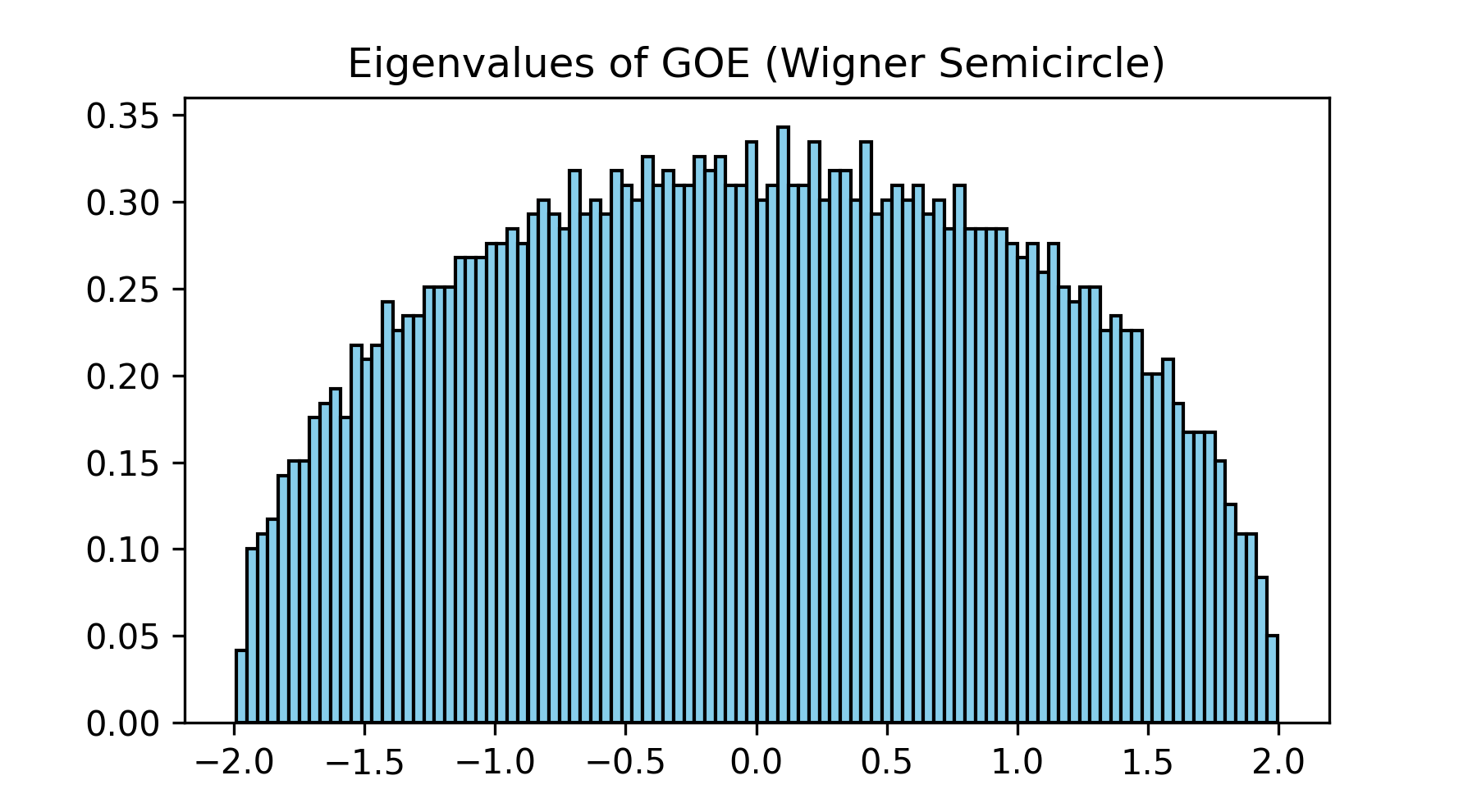

Why Could RMT Solve the Mysteries of Machine Learning?

So, why has this mathematical theory become an indispensable tool for analyzing the generalization performance of machine learning? It is because the "datasets" and the "weight parameters" of neural networks handled in machine learning can be viewed as massive random matrices.

To put the difference simply, while conventional statistical learning theory assumes the worst-case scenario ("no matter how unlucky the data is, the error will not exceed this bound") to obtain an upper bound on the generalization error (Worst-case analysis), RMT uses probabilistic limits to describe the "average behavior" of the generalization error (Average-case analysis). Therefore, the theoretical formulas for generalization error derived using RMT successfully and mathematically rigorously explained the double descent phenomenon in the over-parameterized regime.

Roadmap of This Article

In this article, we will explain in an easy-to-understand manner how this random matrix theory has evolved and become the foundation of modern machine learning, following its historical progression and theoretical breakthroughs:

1. The Era of Independence: The Marchenko-Pastur Law (1967)
2. Breaking the Constraints: Establishing a Solid Theoretical Foundation by Silverstein (1995)
3. Establishment of Deterministic Equivalents (2007-2011): A groundbreaking paradigm shift by Hachem, Loubaton, & Najim (2007) and Rubio & Mestre (2011).
4. Extension to Nonlinear Feature Vectors (Recent years): Theoretical extensions to data with nonlinear correlations by Louart et al.
5. Analysis of Test Risk and Unraveling the "Double Descent" Phenomenon: How RMT solved the mysteries of machine learning.

Now, let's step into the profound world of Random Matrix Theory.

1. Sample Covariance Matrices and the Stieltjes Transform

The primary object of study in high-dimensional data analysis is the Sample Covariance Matrix.

This matrix $\hat{\Sigma}$ is a crucial matrix that represents the variance structure of the data and plays a central role in training and evaluating the performance of machine learning models. In RMT, the primary interest lies in the distribution of eigenvalues when the matrix dimension $p$ becomes large. Let the $p$ eigenvalues of $\hat{\Sigma}$ be $s_1, \dots, s_p$. Its Empirical Spectral Distribution (ESD) can be written as:

However, it is extremely difficult to directly calculate the eigenvalues of a massive random matrix and mathematically determine its distribution function. Here, a powerful analytical tool that supported the development of RMT comes into play: the Stieltjes Transform. The Stieltjes transform $S_\mu(z)$ for a probability measure $\mu$ is defined for a complex number $z \in \mathbb{C} \setminus \mathbb{R}$ as follows:

When this definition is applied to the empirical spectral distribution $\mu_{\hat{\Sigma}}$ of the sample covariance matrix, it can be rewritten into a surprisingly simple matrix form:

This $(\hat{\Sigma} - zI_p)^{-1}$ is called the Resolvent Matrix. In RMT, rather than taking the difficult approach of "calculating eigenvalues directly," we follow a refined route: "find the limit of the trace of the resolvent (the Stieltjes transform), and from there, back-calculate the eigenvalue distribution using complex analysis techniques." Furthermore, when evaluating the test error of machine learning models such as ridge regression, the trace of this resolvent appears directly in the formulas. Therefore, deriving the Stieltjes transform directly translates to predicting machine learning performance.

2. The Era of Independence: The Marchenko-Pastur Law (1967)

In classical statistics, we consider the limit where the number of samples $N_{\mathrm{s}} \to \infty$ while the number of features $p$ remains fixed. In this case, by the law of large numbers, the eigenvalue distribution of $\hat{\Sigma}$ simply converges to the eigenvalues of the population covariance matrix $\Sigma$.

However, in modern machine learning, it is common for the number of features $p$ and the number of samples $N_{\mathrm{s}}$ to be of a similar magnitude. Actually, in such situations, classical statistical theories cannot be applied. Even when the population covariance matrix $\Sigma$ is the identity matrix $I_p$ (where all eigenvalues are $1$), the eigenvalue distribution of $\hat{\Sigma}$ converges to a non-trivial distribution with a certain width.

In 1967, Marchenko and Pastur showed that in the "proportional asymptotic regime," where both the matrix dimension $p$ and the number of samples $N_{\mathrm{s}}$ go to infinity while their ratio $\gamma := p/N_{\mathrm{s}} \in (0, \infty)$ is kept constant, the eigenvalue distribution of this matrix converges to a deterministic limit distribution.

As can be seen from this result, when the number of samples $N_{\mathrm{s}}$ and the number of features $p$ are of similar magnitude, the eigenvalues of the sample covariance matrix $\hat{\Sigma}$ do not concentrate at a single point $\sigma_x^2$. Instead, due to sampling fluctuations, the eigenvalues spread out into a bulk centered around $\sigma_x^2$ with a width of $[\gamma_-, \gamma_+]$. However, if $p$ is sufficiently smaller than $N_{\mathrm{s}}$, the eigenvalues will be narrowly distributed around $\sigma_x^2$, making it consistent with classical statistical theory.

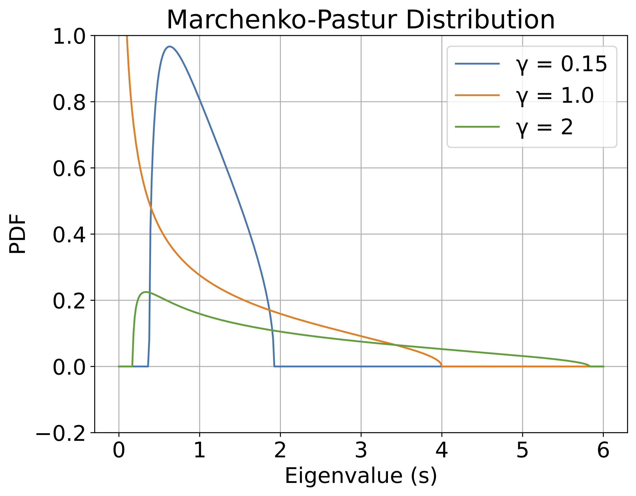
What is noteworthy here is how the distribution changes depending on the dimensional ratio $\gamma := p/N_{\mathrm{s}}$ (the ratio of the number of parameters to the number of samples).

• $\gamma < 1$ (Under-parameterized): Since $p < N_{\mathrm{s}}$, the bulk of the eigenvalues forms a neat mountain away from zero.
• $\gamma = 1$ (Interpolation threshold): Since $p = N_{\mathrm{s}}$, we have $\gamma_- = 0$, resulting in a singularity (peak) where the distribution diverges to infinity near zero. This implies that the smallest eigenvalue of the matrix approaches zero, making it extremely ill-conditioned. This is the direct cause of the "interpolation peak (divergence of error) in double descent," which will be discussed later.
• $\gamma > 1$ (Over-parameterized): Since $p > N_{\mathrm{s}}$, the matrix becomes rank-deficient. As a result, a massive number of exactly zero eigenvalues are generated (the Dirac delta function $\delta(x)$ in the second term of the equation), and the remaining non-zero eigenvalues form a bulk on the right side.

While this result was extremely powerful, it was based on the strong assumption that "all entries are completely independent (the population covariance matrix is $\Sigma = \sigma_x^2 I_p$)." In reality, data generally has complex correlation structures between features, meaning that this assumption of independence could not be applied to the performance analysis of practical machine learning models.

The Brilliance of RMT: Universality

The reason RMT results, including the Marchenko-Pastur Law, boast immense practicality in machine learning lies in their property of Universality. Whether the elements of the data matrix are generated from a neat "Gaussian distribution (normal distribution)" or from a "coin toss (Rademacher distribution)" where $+1$ and $-1$ appear with equal probability, as long as the mean and variance (moments up to the second order) match, the eigenvalue distribution in the limit perfectly aligns with the exact same Marchenko-Pastur Law curve. Because they do not depend on the specific shape of the data distribution (higher-order moments), theoretical formulas hold strong predictive power even for real-world data.

# Simulation of a Wishart matrix (Marchenko-Pastur law)
p, N_s = 500, 1000 # Case where γ = 0.5
X = np.random.randn(p, N_s)
W = np.dot(X, X.T) / N_s
eigvals_W = np.linalg.eigvalsh(W)

# Simulation with coin tosses (Rademacher distribution)
X_rademacher = np.random.choice([-1, 1], size=(p, N_s))
W_rademacher = np.dot(X_rademacher, X_rademacher.T) / N_s
eigvals_W_rademacher = np.linalg.eigvalsh(W_rademacher)

plt.hist(eigvals_W, bins=50, density=True, alpha=0.6, label="Gaussian")
plt.hist(eigvals_W_rademacher, bins=50, density=True, alpha=0.6, label="Rademacher (Coin Toss)")
plt.title("Universality of Marchenko-Pastur Law")
plt.legend()
plt.show()
# Even in a finite experiment, both converge to almost the same distribution (they are completely identical in the limit)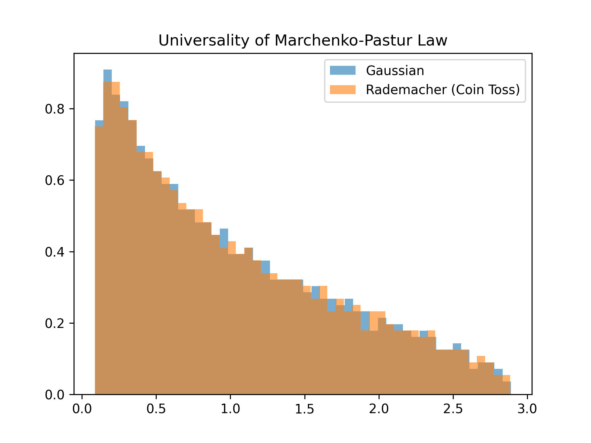

3. Breaking the Constraints: Establishing a Solid Theoretical Foundation by Silverstein (1995)

The standard Marchenko-Pastur Law introduced in Chapter 2 is very beautiful and powerful, but it is often applied to cases where "all features are completely independent (the true population covariance matrix is $\Sigma = \sigma_x^2 I_p$)." However, in real-world image or audio data, complex correlations exist between pixels and features, so the assumption of independence cannot be applied to the analysis of practical machine learning models.

In fact, the original 1967 paper by Marchenko and Pastur already presented the prototype of the equation for cases considering the correlation structure of data. However, its mathematical proof imposed overly strict constraints that were too harsh to apply to real data, such as "the absolute fourth moments of the matrix entries must be finite."

The mathematician who broke through this theoretical wall and completed a solid foundation leading to modern machine learning was Jack Silverstein in his 1995 research. He considered a setting where the data matrix $X$ is generated using the true covariance matrix $\Sigma_p$ as follows:

Here, $Z \in \mathbb{R}^{N_{\mathrm{s}} \times p}$ is a noise matrix where each element is i.i.d. (independent and identically distributed). In this case, the sample covariance matrix can be written as $\hat{\Sigma} = \frac{1}{N_{\mathrm{s}}} \Sigma_p^{1/2} Z^{\mathsf{T}} Z \Sigma_p^{1/2}$. (In the limit as $N_{\mathrm{s}} \to \infty$ with $p$ fixed, $\frac{1}{N_{\mathrm{s}}} Z^{\mathsf{T}} Z$ converges to the identity matrix $I_p$, so the eigenvalue distribution of $\hat{\Sigma}$ converges to that of $\Sigma_p$.)

Silverstein's greatest achievement was completely removing strict constraints like the 4th moment and proving the theorem under the minimal assumption that "each element of the noise matrix $Z$ only needs to have a mean of $0$ and a variance of $1$ (2nd moment)." Specifically, under a natural high-dimensional limit where $p, N_{\mathrm{s}} \to \infty$ (ratio $p/N_{\mathrm{s}} \to \gamma \in (0, \infty)$) and the empirical eigenvalue distribution of the true covariance matrix $\Sigma_p$ converges to some limit distribution $H$, he rigorously showed that the spectral distribution of $\hat{\Sigma}$ converges almost surely (Strong Convergence) to a deterministic limit distribution.

He then proved that the Stieltjes transform $m(z)$ in that limit is the unique solution to the following integral equation:

The brilliance of this result lies in "discarding complete independence of elements and allowing the true correlation structure to be incorporated into the theory as the limit distribution $H$." Even for troublesome data with extreme outliers, as long as the variance can be defined, it was guaranteed that the limit behavior of the eigenvalue distribution could be captured through this self-consistent equation.

However, for practitioners and machine learning engineers, there was still a barrier to putting this abstract "integral form" equation directly onto computers and using it for model performance prediction. This is because the analytical form of the limit distribution $H$ is often unknown.

Nevertheless, the fact established here by Silverstein—that the asymptotic behavior of random matrices can be rigorously described by an equation based on the true correlation structure—provided extremely important inspiration to researchers in the 2000s. Eventually, this idea of an integral equation was reconstructed into a "practical trace-form equation" using the finite-dimensional matrix $\Sigma_p$ as is, which directly connected to a powerful paradigm shift called the "Deterministic Equivalent," explained in the next chapter.

• Silverstein, J. W. (1995). Strong convergence of the empirical distribution of eigenvalues of large dimensional random matrices.

4. Introduction of Deterministic Equivalents (2007-2011)

Thanks to Silverstein's research, it became possible to calculate the "trace (a quantity related to the sum of eigenvalues)" of a sample covariance matrix constructed from correlated data. However, for analyzing actual machine learning algorithms, this was insufficient.

For example, consider Ridge Regression, which adds regularization to linear regression:

The solution that finds the optimal parameter vector $\hat{\boldsymbol{\beta}}$ from the training data $X$ and the target variable $\boldsymbol{y}$ is given in the following closed-form:

When trying to calculate the "test error (generalization error)" on new unseen data using these parameters, you encounter not just a simple Stieltjes transform: $\frac{1}{p} \mathrm{Tr}[(\hat{\Sigma} + \lambda I_p)^{-1}]$, but more complex terms such as:

Such terms could not be analyzed simply by finding the limit of the trace.

The breakthrough came with a groundbreaking paradigm called the "Deterministic Equivalent (DE)," introduced by Walid Hachem et al. in 2007, and Fernando Rubio and Xavier Mestre et al. in 2011.

• DETERMINISTIC EQUIVALENTS FOR CERTAIN FUNCTIONALS OF LARGE RANDOM MATRICES by Walid Hachem, Philippe Loubaton and Jamal Najim (2007)
• Spectral Convergence for a General Class of Random Matrices by Fernando Rubio and Xavier Mestre (2011)

They proved that not only the limit of the trace, but "the inverse matrix itself of a massive random matrix" could be replaced by a mathematically tractable non-random (deterministic) matrix.

In 2011, for correlated data $X = \Sigma^{\frac12} Z$, Rubio and Mestre derived the deterministic equivalent of the resolvent—the core of the ridge regression solution—as the following formula.

[What makes this so powerful?] When attempting to calculate the prediction error of ridge regression, the inverse matrix of a random matrix, $(\hat{\Sigma} + \lambda I_p)^{-1}$, inevitably appears in the equations, causing the analysis to hit a dead end. However, by applying this "deterministic equivalent" formula, the random $\hat{\Sigma}$ can instantly be replaced with the true $\Sigma$ and the scalar $\kappa_\lambda$. This makes it possible to accurately calculate the true performance (such as generalization error) of machine learning algorithms on high-dimensional data using just pen and paper.

5. To the Frontiers of Nonlinearity

Rubio & Mestre's theory was overwhelmingly powerful, but it had a fatal weakness. It required the assumption that "the data generation process must be linear ($X = \Sigma^{\frac12} Z$)." Modern machine learning, such as the generators in Generative Adversarial Networks (GANs) or Random Feature Models, transforms data using highly advanced nonlinear functions. The assumption of linearity completely fails here.

However, recent studies have shattered this wall. For instance, Louart et al. proved that even if the data consists of "Concentrated Feature Vectors" generated through a Lipschitz continuous nonlinear function, Rubio & Mestre's theorem (the linear deterministic equivalent) can be applied exactly as it is (recently, it was shown that similar results hold even under more relaxed conditions). This became the bridge connecting "classical RMT" and "machine learning with modern complex nonlinear models."

The fact that exactly the same deterministic equivalent as Rubio & Mestre holds in the limit, even for highly nonlinear features, powerfully corroborates the Universality of RMT.

• 2018: A Random Matrix Approach to Neural Networks
• 2023: Spectral properties of sample covariance matrices arising from random matrices with independent non identically distributed columns
• 2026: Resolvent convergence for sample covariance matrices with general covariance profiles and quadratic-form control

6. Analysis of Test Risk and Unraveling the "Double Descent" Phenomenon

By obtaining the ultimate weapon known as the Deterministic Equivalent (DE), we became capable of rigorously calculating the test risk (expected prediction error on unseen data) of machine learning models like ridge regression.

The test risk $R_{\lambda, \hat{\Sigma}}$ can be decomposed into three terms: the Bias of the predictive model, the Variance, and the unobservable noise ($\sigma^2$). Applying Rubio & Mestre's theorem and complex analysis techniques to this equation yields the following theorem.

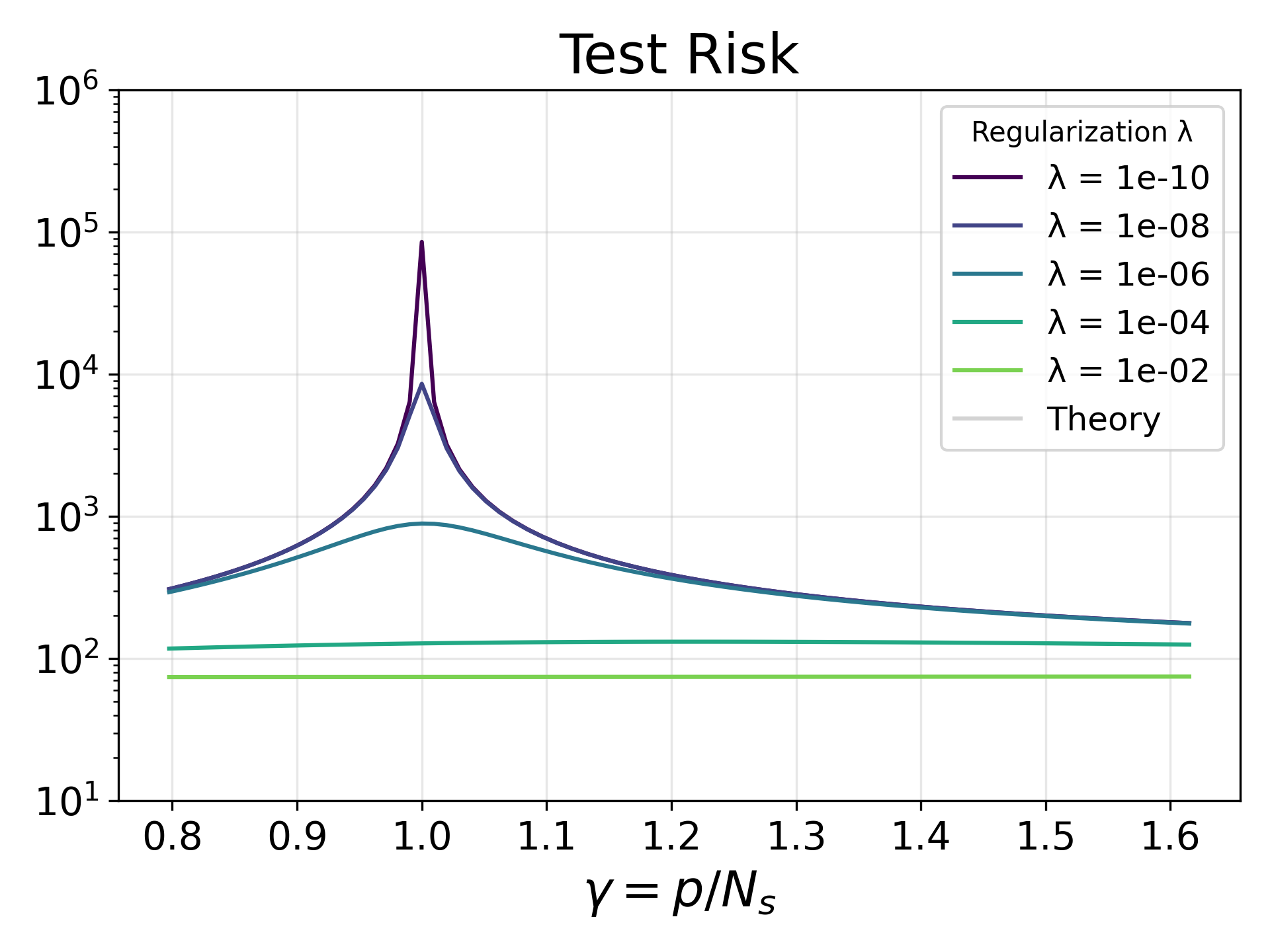
This formula is precisely what completely explains mathematically why the "Double Descent" phenomenon occurs.

In Chapter 2 on the Marchenko-Pastur Law, we confirmed that when the dimensional ratio $\gamma = p/N_{\mathrm{s}}$ is $1$ (i.e., the number of parameters equals the number of samples), an infinite peak forms near zero in the eigenvalue distribution (the matrix becomes extremely ill-conditioned).

Looking at the formula in Theorem 1, when the regularization $\lambda \to 0$ and the number of parameters approaches the number of samples ($p = N_{\mathrm{s}}$), the effective degrees of freedom $\eta_\kappa$ approaches $1$. Then, the denominator of the variance term $(1 - \eta_\kappa)$ approaches zero, causing the variance (sensitivity to noise) to blow up to infinity. The ill-conditioning of the matrix clearly manifests mathematically as the divergence of the test risk (Interpolation peak).

However, as the number of parameters is further increased and we enter the over-parameterized regime ($p \gg N_{\mathrm{s}}$), $\eta_\kappa$ moves away from $1$ again. The expressiveness of the model increases, and optimization progresses in a well-conditioned subspace, causing the test risk to decrease once more. This is the mechanism of Double Descent.

7. The Practical Value of RMT: Predicting Performance Without Model Training

The result of Theorem 1 possesses not only theoretical beauty but also extremely high practical value.

Conventionally, to evaluate the generalization performance of a machine learning model, it was necessary to generate large datasets, repeat model training (involving matrix inversions or optimization loops) many times, and empirically calculate the average test error. This is very costly in terms of computational resources.

However, using this asymptotic test risk formula $R_{\lambda, \Sigma}^{\mathrm{DE}}$, you can completely skip the model training process. By simply substituting the spectral information of the target data's "population covariance matrix $\Sigma$" and the "target vector $\boldsymbol{\beta}_*$" into the self-consistent equations, you can instantly and analytically plot the test risk curve for any data size $N_{\mathrm{s}}$ and regularization parameter $\lambda$.

Despite being a theory predicated on $p, N_{\mathrm{s}} \to \infty$, it has been demonstrated that even in finite, small-scale systems, the theoretical prediction curves given by RMT match empirical test errors astonishingly accurately.

8. Application to Free Probability Theory and Optimization Dynamics

The benefits of RMT are not limited to predicting generalization performance after training is complete. In fact, it also brings a dramatic effect to the analysis of how optimization algorithms like Gradient Descent (GD) converge step by step (learning dynamics).

In the learning process of machine learning models, what determines the shape of the valleys in the loss function (Loss Landscape) is the second derivative, the Hessian matrix $H$. The Hessian of a neural network is often modeled as the sum $H = H_0 + H_1$, where $H_0$ is the "structural term of the data" and $H_1$ is the "noise term from sampling."

Here, a major problem arises. Because matrix multiplication is non-commutative ($AB \neq BA$), we cannot calculate the eigenvalue distribution of the sum of multiple random matrices using the "convolution integral" used for adding regular random variables. The solution to this is Free Probability Theory in RMT.

This spectral analysis of the Hessian enables performance evaluation of algorithms not in the worst-case, but in the average-case. Using RMT's theoretical formulas, it is even possible to derive in advance things like "how many steps Gradient Descent will take to reduce the error by how much (Halting time)" and "the optimal learning rate (step size) to finish learning as fast as possible."

9. Conclusion

Random Matrix Theory began with the analysis of the eigenvalue distribution of simple noise matrices (Marchenko-Pastur Law). Later, realistic correlation structures ($\Sigma$) were incorporated by Silverstein and others, the analytical tool of the Stieltjes transform was refined, and a powerful paradigm called Deterministic Equivalents was established by Hachem, Rubio, Mestre, and others. Today, RMT theories continue to evolve daily, including extensions to nonlinear features by Louart et al.

Currently, Random Matrix Theory has transcended the boundaries of pure mathematics and physics, acting as one of the most powerful theoretical weapons in the analysis of deep learning dynamics and the elucidation of generalization performance.

References

• Marčenko, V. A., & Pastur, L. A. (1967). Distribution of eigenvalues for some sets of random matrices.
• Silverstein, J. W. (1995). Strong convergence of the empirical distribution of eigenvalues of large dimensional random matrices.
• Hachem, W., Loubaton, P., & Najim, J. (2007). Deterministic equivalents for certain functionals of large random matrices.
• Rubio, F., & Mestre, X. (2011). Spectral convergence for a general class of random matrices.
• Louart, C., Liao, Z., & Couillet, R. (2018). A random matrix approach to neural networks.
• Louart, C., & Couillet, R. (2023). Spectral properties of sample covariance matrices arising from random matrices with independent non identically distributed columns.
• Random Matrix Theory and Machine Learning Tutorial