The beautiful stripes of a zebra, the symmetry of a snowflake, the complex indentations of a coastline—. Did you know that these beautiful patterns found in nature, which at first glance seem random and bafflingly complex, are actually generated by extremely simple mathematical formulas and algorithms?

In this article, we will explore the "algorithms of beauty" hidden in the natural world, combining actual visuals with mathematical explanations. Let's experience together the astonishing truth that "the beauty of nature is born from the repetition of simple rules."

1. Turing Patterns: Equations that Draw the Patterns of Life

How are the regular patterns (spots and stripes) seen on the surfaces of animals formed? Alan Turing, the father of modern computer science, challenged this mystery with a mathematical approach.

He used mathematical formulas to show that in the process where two types of chemicals (an activator and an inhibitor) "react" while "diffusing," spatial wave patterns spontaneously emerge. This is known as the reaction-diffusion equation.

Simulating Turing Patterns with Python

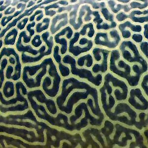
Let's actually calculate the reaction-diffusion equation (using the widely used Gray-Scott model here) using Python. By running the following code, you can see how a complex pattern resembling a living creature's skin emerges from the iteration of simple formulas.

1import numpy as np
2import matplotlib.pyplot as plt
3from matplotlib.colors import LinearSegmentedColormap
4
5def laplacian(Z):
6    # Calculate the spatial spread (Laplacian) from top, bottom, left, and right cells
7    return (np.roll(Z, 1, axis=0) + np.roll(Z, -1, axis=0) +
8            np.roll(Z, 1, axis=1) + np.roll(Z, -1, axis=1) - 4 * Z)
9
10# ★ Crucial part! Parameters for creating a labyrinth pattern
11Du, Dv = 0.16, 0.08  # Diffusion coefficients remain the same
12F, k = 0.042, 0.061  # Changing the balance of F and k creates a labyrinth pattern
13iterations = 10000   # Increase the number of steps to spread the pattern across the screen
14size = 200           # Increase size to represent the fine details of the mesh
15
16# Setup initial state
17U = np.ones((size, size))
18V = np.zeros((size, size))
19
20# Scatter random "seeds" across the screen (to let the pattern grow globally)
21np.random.seed(42) # Seed for reproducibility
22U += 0.05 * np.random.random((size, size))
23V += 0.05 * np.random.random((size, size))
24
25# Place initial triggers near the center
26r = 20
27U[size//2-r:size//2+r, size//2-r:size//2+r] = 0.50
28V[size//2-r:size//2+r, size//2-r:size//2+r] = 0.25
29
30# Time evolution calculation
31for i in range(iterations):
32    Lu = laplacian(U)
33    Lv = laplacian(V)
34    
35    uvv = U * V * V
36    
37    U += Du * Lu - uvv + F * (1 - U)
38    V += Dv * Lv + uvv - (F + k) * V
39
40# ★ Create an original colormap resembling the hues of a pufferfish
41colors = ["#132226", "#2c4a45", "#81a166", "#d9e8b3"] # Dark green to bright yellow-green
42puffer_cmap = LinearSegmentedColormap.from_list("puffer", colors)
43
44# Generate and display the image
45plt.figure(figsize=(6, 6))
46plt.imshow(V, cmap=puffer_cmap, interpolation='bicubic')
47plt.axis('off')
48plt.title("Labyrinth Pattern (Pufferfish Style)", fontsize=14)
49plt.tight_layout()
50plt.show()

2. Fractals: Infinitely Continuing "Self-Similarity"

Another important pattern in the natural world is the fractal. Ria coasts, snowflakes, the branching of blood vessels, etc., possess "self-similarity," meaning that as you zoom in on the whole, a part of it reveals the exact same shape as the whole again.

As a prime example, let's look at the "Romanesco broccoli," a beautiful fractal that naturally exists.

Additionally, the "Mandelbrot set," the most famous fractal in the mathematical world, is born from a surprisingly simple recurrence relation of complex numbers:

When this simple calculation is repeated infinitely, plotting the initial values of $c$ for which the value of $z$ does not diverge reveals that breathtaking, infinite geometric figure.

Drawing the Mandelbrot Set with Python

Let's actually calculate this figure using Python.

1import numpy as np
2import matplotlib.pyplot as plt
3
4def generate_mandelbrot(width, height, x_min, x_max, y_min, y_max, max_iter):
5    # Create a grid on the complex plane
6    x = np.linspace(x_min, x_max, width)
7    y = np.linspace(y_min, y_max, height)
8    X, Y = np.meshgrid(x, y)
9    C = X + 1j * Y
10    Z = np.zeros_like(C)
11    
12    # Array to record the number of iterations until divergence
13    escape_time = np.zeros(C.shape, dtype=int)
14    mask = np.ones(C.shape, dtype=bool)
15
16    for i in range(max_iter):
17        Z[mask] = Z[mask]**2 + C[mask]
18        
19        # Consider it diverged if it exceeds the threshold (radius 2)
20        diverged = np.abs(Z) > 2
21        escape_time[diverged & mask] = i
22        mask[diverged] = False
23
24    return escape_time
25
26# Generate and display the image
27image = generate_mandelbrot(800, 800, -2.0, 0.5, -1.25, 1.25, 100)
28plt.imshow(image, cmap='magma', extent=[-2.0, 0.5, -1.25, 1.25])
29plt.axis('off')
30plt.show()

3. The Game of Life: Complex Systems Born from Simple Rules

The last concept we will introduce is the Game of Life, devised by the British mathematician John Conway in 1970. This is a type of computational model called a "cellular automaton," where cells on a grid resembling a Go board determine their life or death in the next generation based on the state (alive or dead) of their 8 neighboring cells.

There are only four simple rules:

1. Birth: If a dead cell has exactly 3 living neighbors, it becomes alive.
2. Survival: If a living cell has 2 or 3 living neighbors, it stays alive.
3. Underpopulation: If a living cell has 1 or fewer living neighbors, it dies of underpopulation.
4. Overpopulation: If a living cell has 4 or more living neighbors, it dies of overpopulation.

From just these four rules, life-like behaviors that seem almost intentional are born, such as "gliders" that continuously move on their own, or "glider guns" that infinitely spawn cells.

Conclusion

The beauty of the natural world is not meticulously painted stroke by stroke by God, but rather the result of emergence woven by "simple physical rules (mathematical formulas) and iterative calculations (algorithms)."

Learning mathematics and programming is not just for building apps or doing calculations. It is a powerful tool to understand "how the world works" and to recreate its beauty with your own hands through simulations.

The next time you see a pattern in nature, try to think about the mathematical formulas and algorithms hidden within it. The world you are so used to seeing might begin to look like a brand-new work of art.